uncertainly

  • The nonabelian FFT over finite fields

    Introduction

    The discrete Fourier transform is a powerful tool that allows us to translate signals on a space in the time domain to a representation on the frequency domain. There are many variations of this transform, and this post will focus on what happens when we generalize the field we’re working over from the complex numbers to finite fields. We’ll cover the basics of finite fields, the definitions of the transforms, and algorithms to quickly compute them.

    In general, there will be two parameters which we can modify to obtain different variations: the field and the group. The classical DFT is the Fourier transform of the cyclic group over the complex numbers.

    In this article, we will consider both modifications by working over nonabelian groups such as the dihedral group and symmetric group rather than the cyclic group, and we will work over a finite field rather than the complex numbers.

    The Classical Fourier Transform

    The DFT is a discretization of a continuous transform that was discovered in the early 19th century by Jean-Baptiste Joseph Fourier. In particular, he used this to study PDEs that arise naturally in heat flow in a pipe. The Fourier transform takes a function in space, e.g. a distribution of heat in a linear rod, and maps the function to a frequency space as follows:

    \[
    \mathcal{F}: f(x) \mapsto \int_{-\infty}^{\infty} f(x)e^{-2\pi i \xi x}\,dx
    \]

    Often we’ll denote the function \(\mathcal{F}(f)(\xi)=\hat{f}(\xi)\). Note that the input variable is now \(\xi\) rather than \(x\), which is deliberate. \(\xi\) is said to reside in the frequency domain whereas \(x\) is in the time domain or in this case the spatial domain. Note that \(x\) is real, while the output of the transform is generally complex. One of the equations which motivated Fourier’s work is the heat equation, given by

    \[
    \frac{\partial u}{\partial t}=\alpha\frac{\partial^2u}{\partial x^2}.
    \]

    The function \(u:=u(x,t)\) depends on both space and time. For simplicity, let’s suppose we have periodic boundary conditions so that \(u(0,t)=u(L,t)\) and \(u_x(0,t)=u_x(L,t)\). Assume the ansatz that the function is separated so that \(u(x,t)=X(x)T(t)\), a product of a spatial function and a time function. This gives a pair of ODEs so that \(T’=-\alpha\lambda T\) and \(X”=-\lambda X\). For \(\lambda=(2\pi n/L)^2\), we obtain the mode

    \[
    u_n(x,t)=e^{2\pi i n x/L}e^{-\alpha(2\pi n/L)^2t}.
    \]

    Note that periodicity has forced the solution to depend on the discrete parameter \(n\).

    In this case, since the function is periodic, define the Fourier transform as

    \[
    \hat{f}(n)=\int_0^L f(x)e^{-2\pi i n x/L}\,dx.
    \]

    Since the PDE is linear, a general solution can be expressed as a linear superposition of the individual solutions.

    \[
    u(x,t)=\sum_{n=-\infty}^{\infty}c_ne^{2\pi i n x/L}e^{-\alpha(2\pi n/L)^2t},
    \]

    where \(c_n=\frac{1}{L}\hat{f}(n)\).

    Thus one can think of the general solution as having modes which depend on \(n\), and each mode corresponds to an eigenfunction which describes the distribution of heat in that mode, and over time the heat dissipates with exponential decay. Since we enforced periodic boundary conditions, one can imagine the heat is sloshing around inside a circular metal tube, cooling down over time.

    In real applications, it is often the case that rather than having an infinitely fine, continuous set of measurements we only have a sequence of concrete measurements of some fixed number \(N\). How should the Fourier transform generalize to this case, and what types of problems would it solve?

    The Discrete Fourier Transform

    Imagine that we have a discrete set of measurements, a signal, which is given by \(\mathbf{x}(n):=x_n\in\mathbb{R}\). Thus, for each discrete \(n\) we have a real number. We discretize the integral using summation to obtain the discrete Fourier transform or DFT:

    \[
    \mathcal{F}:\mathbf{x}\mapsto
    \left(\sum_{n=0}^{N-1}x_ne^{-2\pi i kn/N}\right)_{k=0}^{N-1}.
    \]

    That is, \(\mathcal{F}(\mathbf{x})(k):=\hat{\mathbf{x}}(k)\). In other words, given a vector \(\mathbf{x}\), we obtain a new vector with components depending on \(k\) rather than \(n\), and those components we think of as frequencies depending on the discrete parameter \(k\).

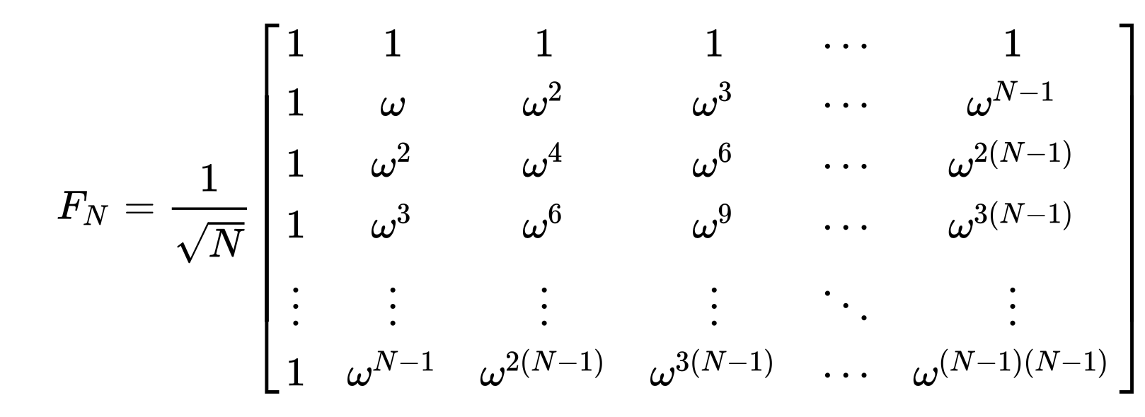
    A couple things are happening here. The first thing to note is that this is a linear operator. In fact, this gives us a linear map from \(\mathbb{R}^N\rightarrow\mathbb{C}^N\). In practice, it will be useful to allow complex inputs as well as real inputs, so we obtain a linear map on the same field, \(\mathcal{F}:\mathbb{C}^N\rightarrow\mathbb{C}^N\). Using the standard basis, this transformation can be represented as an \(N\times N\) matrix.

    \[
    F_N=
    \begin{pmatrix}
    1 & 1 & 1 & \cdots & 1 \\
    1 & \omega & \omega^2 & \cdots & \omega^{N-1} \\
    1 & \omega^2 & \omega^4 & \cdots & \omega^{2(N-1)} \\
    1 & \omega^3 & \omega^6 & \cdots & \omega^{3(N-1)} \\
    \vdots & \vdots & \vdots & \ddots & \vdots \\
    1 & \omega^{N-1} & \omega^{2(N-1)} & \cdots & \omega^{(N-1)(N-1)}
    \end{pmatrix},
    \qquad \omega=e^{-2\pi i/N}.
    \]

    The other important thing to note is that now that we are in the discrete realm, we could think about the index set of our vectors. It is a discrete list of numbers \(n,k\in 0,1,\ldots,N-1\). Since there are no boundary conditions a priori, it makes sense to imagine that this sequence extends to \(n=N\), but that \(x_N=x_0\), and so on so that we automatically have a periodic sequence with periodic boundary conditions.

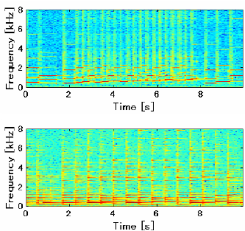
    Where is this used? Well, everywhere is the answer. More specifically, it’s used in signal processing. In that case, the indexing set is taken to represent a discrete set of time measurements, and the signals are the magnitude and phase of something you’re measuring. One could measure, say, an audio signal which is sampled at some sampling rate. Then the DFT can be used to break the signal into components. This is especially useful if you’re trying to understand the pitches and frequencies contained in a musical sound. A spectrogram is obtained by taking a small piece of the time domain, performing the DFT, and then repeating in chunks to see which frequencies are approximately present for each time block. See Figure 1 to see a spectrogram for a flute and piano.
    Sound spectrogram comparing a flute and piano.
    Figure 1. Sound spectrogram; top: flute, bottom: piano. Colors correspond to the magnitude: red is strong and blue is weak.

    Now that we’re comfortable with the DFT, we can think a little harder about the index set. Since the signal is periodic, we have some \(x_n\) for each \(n\in\mathbb{Z}\). Since it repeats, it’s better to think of the signal as simply being defined on \(\mathbb{Z}/N\mathbb{Z}\), the cyclic group of order \(N\). A finite list of outputs depending on an input can also be thought of as a function, so now we can think of \(\mathbf{x}:\mathbb{Z}/N\mathbb{Z}\rightarrow\mathbb{C}\). Thus, \(\mathcal{F}\) is really about transforming one function defined on a cyclic group to another function defined on a cyclic group.

    Let’s denote the cyclic group by \(C_N=\mathbb{Z}/N\mathbb{Z}\). We can now use the fancier notation \(\mathcal{F}:\mathbb{C}[C_N]\rightarrow\mathbb{C}[C_N]\). The algebraic object \(\mathcal{C}_N=\mathbb{C}[C_N]\) is called the group algebra of the cyclic group, and gives us a different perspective to bear on this transform. First note that \(\mathcal{C}_N\) is a vector space of dimension \(N\) over \(\mathbb{C}\). Given two elements \(a,b\) of \(\mathcal{C}_N\), we can multiply them as follows. Let \(a=\sum_i a_i\alpha^i\) and \(b=\sum_j b_j\alpha^j\). Then

    \[
    a\cdot b=\sum_{i,j}a_ib_j\alpha^{i+j},
    \]

    where again we take the indices \(i\) to be defined modulo \(N\), and \(\alpha\in C_N\) is a generator of the cyclic group. This multiplication is associative and is the reason we call this an algebra.

    The next thing to notice is that every finite group has a collection of representations. Note further that \(C_N\) is an abelian group, so that its irreducible representations are one dimensional. Namely, for each \(k\) we have the map \(\rho_k:\mathbb{Z}/N\mathbb{Z}\rightarrow\mathbb{C}^{\times}\) given by \(\rho_k(n)=e^{2\pi i kn/N}\).

    A representation means that the additive group law on \(\mathbb{Z}/N\mathbb{Z}\) is reflected in the multiplicative structure \(\mathbb{C}^{\times}\), so that \(\rho_k(n_0+n_1)=\rho_k(n_0)\rho_k(n_1)\). We can also recognize that \(\rho_k(n)\) is always an \(N^{th}\) root of unity. That is, \(\rho_k(n)\) lies on the unit circle \(S^1\) in the complex plane.

    One dimensional representations of a group are called characters. Write \(\chi_k(n)=\rho_k(n)\). Then we can rewrite our Fourier transform as

    \[
    \mathcal{F}:\mathbf{x}\mapsto
    \left(\sum_{n=0}^{N-1}x_n\overline{\chi_k(n)}\right)_{k=0}^{N-1}.
    \]

    Thus, we can now express what the DFT is in entirely new language.

    Definition. The discrete Fourier transform (DFT) is the linear map from \(\mathcal{C}_N\) to \(\mathcal{C}_N\) defined by summing the components of a signal \(x_n\) against the complex conjugate of the \(k^{th}\) character \(\chi_k(n)\) over \(n\).

    This immediately hints at a generalization: why not replace the cyclic group by a more complicated, nonabelian group? It turns out there is nothing stopping us, but we will have to be more careful about the definition, and work with representations which are no longer characters, i.e. their dimension is greater than one. In other words, we need to deal with representations that are matrices rather than just numbers.

    The Nonabelian Fourier Transform

    The simplest nonabelian group after the cyclic group is arguably the dihedral group. (There are other natural examples, such as the Heisenberg p-groups over a finite field, but the dihedral group already has representations only in dimensions 1 and 2.) The dihedral group is the symmetries of a regular polygon with \(N\) vertices in the plane, so we have both a rotation \(r\) of order \(N\), as well as a flip symmetry \(s\) of order 2. In this convention, \(D_N\) has order \(2N\).

    \[
    D_N=\langle r,s\mid r^N=s^2=e,\ srs^{-1}=r^{-1}\rangle.
    \]

    The dihedral group also has representations. One can think of a representation as a way for a group to act on a vector space. That is, given a representation \(\rho\), we can let the symmetries of the group act as \(g\cdot v=\rho(g)v\). Thus, we need \(\rho\) to map every group element \(g\) to a matrix. If the dimension of the vector space is \(d\), then this will be a \(d\times d\) matrix.

    For the dihedral group, there will be representations of dimensions 1 and 2. The one dimensional characters are analogous to the characters we mentioned for the cyclic group. We can think of the two dimensional representations as \(2\times 2\) matrices which encode rotations and reflections in the plane. The behavior is different for \(N\) even and \(N\) odd.

    \[
    N\text{ odd}:\quad
    \chi_+,\chi_-,\rho_k
    \quad\text{for}\quad
    k=1,\ldots,(N-1)/2,
    \]

    \[
    N\text{ even}:\quad
    \chi_1,\chi_2,\chi_3,\chi_4,\rho_k
    \quad\text{for}\quad
    k=1,\ldots,N/2-1.
    \]

    Now that we are familiar with the group algebra of a cyclic group, we can do something very straightforward: replace \(C_N\) by \(D_N\). That is, we should study the group algebra \(\mathcal{D}_N=\mathbb{C}[D_N]\). As before, we can multiply \(a,b\in\mathcal{D}_N\) via

    \[
    \left(\sum_g a_gg\right)
    \left(\sum_h b_hh\right)
    =
    \sum_{g,h}a_gb_hgh.
    \]

    You think of these as generalizations of polynomials, where we have replaced monomials like \(x^i\) with group elements \(g\). In this generality, we can think of how the group algebra decomposes when we allow a group \(G\) to act on \(\mathbb{C}[G]\). In particular, since \(\mathbb{C}[G]\) is a ring, we can extend the action of \(G\) to an action of \(\mathbb{C}[G]\), thus we can consider the group algebra as a module over itself. The punchline is that it decomposes very nicely (over the complex numbers) into pieces which are indexed by the representations. In fact, it decomposes into pieces which are endomorphism algebras of the vector space associated to the representation. In simpler terms, these are \(d\times d\) matrix algebras. The semisimplicity statement is known as Maschke’s theorem; together with the Artin–Wedderburn theorem, it gives the decomposition we need:

    Theorem (Maschke). Let \(G\) be a finite group and \(\mathbb{C}[G]\) its group algebra. Then \(\mathbb{C}[G]\) is semisimple: every \(\mathbb{C}[G]\)-module decomposes as a direct sum of irreducible submodules. Consequently, by the Artin–Wedderburn theorem, if \(\{\rho_1,\ldots,\rho_r\}\) is a complete set of pairwise non-isomorphic irreducible representations of \(G\), with \(d_i=\dim\rho_i\), then

    \[
    \mathbb{C}[G]\cong
    \bigoplus_{i=1}^{r}\operatorname{Mat}_{d_i}(\mathbb{C})
    \]

    as \(\mathbb{C}\)-algebras, where the isomorphism is the linear extension of \(g\mapsto(\rho_1(g),\ldots,\rho_r(g))\). In particular,

    \[
    |G|=\sum_{i=1}^{r}d_i^2.
    \]

    Thus, this theorem is telling us how to break down the group algebra using representations. There is one summand, one block, for each representation. It may be helpful to think of a representation as a sort of generalization of the notion of frequency.

    Recall our earlier definition of the Fourier transform. It turns out the linear isomorphism provided by this theorem is exactly the gadget we need.

    Definition. The DFT for nonabelian groups is the linear map \(\mathbb{C}[G]\rightarrow\bigoplus_\rho\operatorname{End}(V_\rho)\) given by \(\hat{f}(\rho)=\sum_g f(g)\rho(g)\).

    Note that an endomorphism is a linear map from a vector space to itself. In this case, once we choose a basis, \(\operatorname{End}(V_\rho)\) is \(\operatorname{Mat}_{d\times d}\), the vector space of \(d\times d\) matrices, and \(V_\rho\) is the vector space corresponding to the representation. For the dihedral group, again, we are only getting \(1\times 1\) matrices (numbers) and \(2\times 2\) matrices.

    The subtle thing to note is that \(\hat{f}(\rho)\) is a \(d\times d\) matrix, i.e. it is no longer just a number. It has \(d^2\) components. It is also important to note that there is no basis on the right hand side which is independent of our choices. For the left hand side, the group itself forms a natural basis for \(\mathbb{C}[G]\), but on the right hand side we must choose a concrete model and a basis for each representation before flattening the \(d\times d\) matrices.

    Once we know the representations of a group, it is in principle possible to use this definition to compute the DFT.

    This construction works for any finite group, in particular the symmetric group on \(N\) symbols, \(S_N\). The symmetric group is the group of permutations of \(N\) items \(\{1,\ldots,N\}\). It is a nonabelian group of order \(N!\). Its representation theory is much more complicated than that of the dihedral group. For now, we merely note that the representations are indexed by partitions \(\lambda\) of \(N\). The dimensions of these representations we denote by \(d_\lambda\), and they are given by an explicit formula called the hook length formula. We’ll denote the group algebra of the symmetric group by \(\mathcal{S}_N=\mathbb{C}[S_N]\).

    Working Over a Finite Field

    The constructions we built thus far share an interesting property, namely that they are all defined using complex numbers. However, we can ask: is there anything inherent in the complex numbers preventing us from extending these definitions to other fields of interest, namely finite fields?

    If you haven’t encountered them before, finite fields are beautiful objects which have an entirely self-contained arithmetic, but only use a finite set of “numbers”. That is, one can add, subtract, multiply, and divide without leaving this finite set. The first example of a finite field, and perhaps the most useful, is the integers modulo a prime number, \(\mathbb{Z}/p\mathbb{Z}\). In a finite field, we need to divide by any nonzero number, which is what forces the modulus to be a prime. For a non-prime modulus \(m\), we could factor \(m=m_0m_1\) and then in the ring \(\mathbb{Z}/m\mathbb{Z}\), we have \(m_0m_1=m\equiv 0\text{ mod }m\).

    Thus, for each prime we have a finite field. The characteristic of a finite field is \(p\), which is the smallest number such that \(p\equiv 0\) in the field. Every finite field has size a prime power \(q=p^r\) for some \(r\), and for each prime power there is a unique finite field up to isomorphism. For our purposes, the most important property is that the set of nonzero elements of the field \(\mathbb{F}_q^\times\) forms a cyclic group of order \(q-1\) (everything except zero).

    We now ask what happens when we replace our favorite field \(\mathbb{C}\) with our next favorite field \(\mathbb{F}_q\)? The definition of a group algebra carries over right away, so \(\mathbb{F}_q[G]\) is still a well-defined ring. The next theorem we’d be interested in is Maschke’s theorem. It turns out that the theorem holds exactly, as long as \(p\nmid |G|\). That is, when the characteristic divides the order of the group things are nowhere near as nice, and this is the field of modular representation theory. For the remainder of the article, we’ll assume \(p\nmid |G|\). We should also note that semisimplicity alone does not guarantee that every block is a matrix algebra over \(\mathbb{F}_q\) itself: for that, \(\mathbb{F}_q\) must be a splitting field for \(G\). The hypotheses in the examples below ensure that the representations we use are defined over our chosen field.

    The final ingredient we need is some notion of a root of unity. Over the complex numbers, we used \(\omega=e^{2\pi i/N}\). The property we’re after is that \(\omega^N=1\). In other words, is there a solution to \(x^N=1\) in \(\mathbb{F}_q\)? This depends on the factorization of \(x^N-1\) in characteristic \(p\), but the punchline is that a primitive \(N^{th}\) root of unity exists in \(\mathbb{F}_q\) whenever \(N\mid q-1\). If \(\gcd(N,p)=1\) but \(N\nmid q-1\), we can pass to a sufficiently large finite extension to obtain one. If \(p\mid N\), however, no finite extension of characteristic \(p\) contains a primitive \(N^{th}\) root of unity.

    Subject to these hypotheses, there is nothing preventing us from replacing \(\mathbb{C}\) by \(\mathbb{F}_q\).

    The Number Theoretic Transform

    There are situations in which we wish to encode data rather than measure signals. In such cases, we replace a signal over the complex numbers with a list of elements in a finite field. Rather than considering functions \(\mathbb{Z}/N\mathbb{Z}\rightarrow\mathbb{C}\) as we have above, we instead consider functions \(\mathbb{Z}/N\mathbb{Z}\rightarrow\mathbb{F}_q\), and here we will also have \(N\mid q-1\).

    The DFT we defined above extends naturally to this case. We can simply replace \(\omega=e^{2\pi i/N}\) with \(\tilde{\omega}\in\mathbb{F}_q\), a primitive \(N^{th}\) root of unity in the finite field. That is, \(\tilde{\omega}^N=1\) in \(\mathbb{F}_q\). Thus our Fourier transform is just

    \[
    \mathcal{F}:\mathbf{x}\mapsto
    \left(\sum_{n=0}^{N-1}x_n\tilde{\omega}^{kn}\right)_{k=0}^{N-1}.
    \]

    This gives us a map \(\mathbb{F}_q^N\rightarrow\mathbb{F}_q^N\). In particular, we may choose \(q=p\) and work over the finite field \(\mathbb{Z}/p\mathbb{Z}\). Doing so yields the number theoretic transform, often abbreviated NTT.

    The number theoretic transform is used heavily in cryptography. In that case, there are certain polynomial rings which look morally like \(\mathbb{F}_q[x]/(x^N-1)\), which is isomorphic to the group ring of a cyclic group over a finite field. Some lattice-based cryptosystems instead use the negacyclic ring \(R_q=\mathbb{F}_q[x]/(x^N+1)\). The choice of ring is tied to both security and efficiency; multiplication in the negacyclic ring can also be accelerated using an NTT when the field contains the appropriate roots of unity. In either case the degree is at most \(N-1\), thus we can think of the coefficients as a list of \(N\) elements of \(\mathbb{F}_q\).

    Part of post-quantum cryptography is multiplying these polynomials, and we would like it to be as fast as possible. This begs the question: is there a fast version of the discrete Fourier transform, and in particular the number theoretic transform? Indeed, there is.

    The Fast NTT

    Again, note the usual NTT is given by \(\hat{x}_k=\sum_{n=0}^{N-1}x_n\tilde{\omega}^{nk}\). For the radix-2 algorithm, we require \(N\) to be a power of two. We split the sum into its even and odd terms as

    \[
    \hat{x}_k
    =
    \sum_{m=0}^{N/2-1}x_{2m}(\tilde{\omega}^2)^{mk}
    +
    \tilde{\omega}^k
    \sum_{m=0}^{N/2-1}x_{2m+1}(\tilde{\omega}^2)^{mk}.
    \]

    Note that each sum is itself an NTT of length \(N/2\) if we recognize that the root of unity we’re using is \(\tilde{\omega}^2\) in place of \(\tilde{\omega}\). The factor \(\tilde{\omega}^k\) is called a twiddle factor. We can then proceed recursively in exactly the same manner as Cooley–Tukey.

    A major difference between the DFT and NTT is that here we are working in exact arithmetic – there are no floating point errors because we’re using finite-field arithmetic.

    I have implemented the underlying NTT in Rust in the ntt crate.

    The FFT of the Dihedral Group Over a Finite Field

    We are now in a position to combine the two generalizations we have been developing. We have replaced the cyclic group by a nonabelian group, and we have replaced the complex numbers by a finite field. Let’s start with the dihedral group, where the structure of the algorithm is especially transparent.

    Recall that every element of \(D_N\) is either a rotation \(r^j\) or a reflection \(sr^j\). Thus, a function \(f:D_N\rightarrow\mathbb{F}_q\) can be written as two lists of field elements,

    \[
    a_j=f(r^j),
    \qquad
    b_j=f(sr^j),
    \qquad
    0\leq j<N.
    \]

    Assume that the characteristic \(p\) does not divide \(2N\), and that \(\mathbb{F}_q\) contains a primitive \(N^{th}\) root of unity \(\omega\). Maschke’s theorem then applies just as it did over \(\mathbb{C}\).1 In particular, the Fourier transform breaks \(\mathbb{F}_q[D_N]\) into blocks corresponding to the irreducible representations of \(D_N\). The one dimensional representations give numbers, and the two dimensional representations give \(2\times 2\) matrices.

    For the two dimensional representation indexed by \(k\), we can choose

    \[
    \rho_k(r^j)=
    \begin{pmatrix}
    \omega^{kj} & 0\\
    0 & \omega^{-kj}
    \end{pmatrix},
    \qquad
    \rho_k(sr^j)=
    \begin{pmatrix}
    0 & \omega^{-kj}\\
    \omega^{kj} & 0
    \end{pmatrix}.
    \]

    If we plug these matrices into the definition of the nonabelian DFT, we obtain

    \[
    \hat{f}(\rho_k)=
    \begin{pmatrix}
    \displaystyle\sum_{j=0}^{N-1}a_j\omega^{kj}
    &
    \displaystyle\sum_{j=0}^{N-1}b_j\omega^{-kj}\\
    \displaystyle\sum_{j=0}^{N-1}b_j\omega^{kj}
    &
    \displaystyle\sum_{j=0}^{N-1}a_j\omega^{-kj}
    \end{pmatrix}.
    \]

    This formula is the punchline. Each entry of the matrix is an ordinary number theoretic transform of either the rotation data \(a\) or the reflection data \(b\). Frequencies with a negative exponent are already present at the corresponding index \(N-k\). Thus the nonabelian transform can be assembled from cyclic NTTs, followed by a small amount of bookkeeping which places their outputs into \(2\times 2\) matrices. The one dimensional pieces appear at the exceptional frequencies \(0\), and also \(N/2\) when \(N\) is even.

    This is a satisfying example because the noncommutativity of the dihedral group does not destroy the FFT we already know. It merely changes the shape of the answer. For the cyclic group, every frequency is a number. For the dihedral group, most frequencies are \(2\times 2\) matrices. Since the cyclic transforms cost \(O(N\log N)\) operations and assembling the matrices costs only \(O(N)\), the entire dihedral transform also costs \(O(N\log N)\) rather than the \(O(N^2)\) operations required by the definition.

    It also gives us fast multiplication in the group algebra. The Fourier transform turns multiplication in \(\mathbb{F}_q[D_N]\) into ordinary multiplication inside each block. We transform two elements, multiply the one dimensional blocks as numbers and the two dimensional blocks as matrices, and then apply the inverse transform. This is exactly the same pattern as polynomial multiplication using the NTT, except that “pointwise multiplication” has become blockwise matrix multiplication.

    I have implemented the dihedral transform in the fft-dihedral crate. There is also a Python implementation for those who would like to experiment with the transform directly.

    The FFT of the Symmetric Group Over a Finite Field

    The dihedral group is a good first nonabelian example because its irreducible representations have dimension at most two. We can now ask what happens for a group whose representations are considerably more complicated. The natural next example is the symmetric group \(S_N\).

    As mentioned above, the irreducible representations of \(S_N\) are indexed by partitions \(\lambda\) of \(N\). If \(\rho_\lambda\) has dimension \(d_\lambda\), then the Fourier transform of a function \(f:S_N\rightarrow\mathbb{F}_q\) contains one \(d_\lambda\times d_\lambda\) matrix for each partition:

    \[
    \hat{f}(\lambda)
    =
    \sum_{\sigma\in S_N}f(\sigma)\rho_\lambda(\sigma).
    \]

    We will assume the characteristic \(p\) is greater than \(N\). In particular, \(p\) does not divide \(N!\), so Maschke’s theorem applies to \(\mathbb{F}_q[S_N]\). In this range the representations we need can be constructed over the finite field, and we again obtain a decomposition.

    \[
    \mathbb{F}_q[S_N]
    \cong
    \bigoplus_{\lambda\vdash N}
    \operatorname{Mat}_{d_\lambda}(\mathbb{F}_q).
    \]

    The dimensions still satisfy \(\sum_{\lambda\vdash N}d_\lambda^2=N!\), as they must: the matrices on the right contain exactly as many field elements as there are permutations on the left.

    Of course, the definition alone does not give a fast algorithm. If we computed every matrix entry by summing over all \(N!\) permutations, we would be throwing away nearly all of the structure of the symmetric group. The relevant structure is the chain of subgroups

    \[
    S_1\subset S_2\subset\cdots\subset S_N.
    \]

    When an irreducible representation of \(S_N\) is restricted to \(S_{N-1}\), it decomposes according to a particularly clean rule: remove one box from the partition \(\lambda\) in every valid way. This is called the branching rule. Even better, each smaller representation appears at most once. The partitions therefore form a branching diagram, and the FFT proceeds recursively down this diagram.

    To see the basic idea, choose representatives \(g_j\) for the cosets of \(S_{N-1}\) in \(S_N\). Any element \(f\in\mathbb{F}_q[S_N]\) can be split into \(N\) smaller pieces,

    \[
    f=\sum_{j=1}^{N}g_jf_j,
    \qquad
    f_j\in\mathbb{F}_q[S_{N-1}].
    \]

    We first compute the transforms of the \(f_j\) recursively. The branching rule tells us how those smaller matrix blocks sit inside a representation of \(S_N\), and multiplication by \(\rho_\lambda(g_j)\) puts them into the correct position. In this way, the transform on \(S_N\) is assembled from transforms on \(S_{N-1}\) rather than computed from scratch. Young’s seminormal representations are especially useful here because adjacent transpositions act by sparse matrices, making these assembly steps fast.

    The story is more elaborate than it was for the dihedral group, but the principle is the same. We find a subgroup whose Fourier transform we already understand, separate the larger group into pieces indexed by its cosets, and use the way representations restrict to that subgroup to put the pieces back together. For the cyclic group, this recursion is the familiar even and odd split of Cooley–Tukey. For the symmetric group, it is controlled by partitions and the branching rule.

    Once again, multiplication in the group algebra becomes blockwise matrix multiplication:

    \[
    \widehat{fg}(\lambda)
    =
    \hat{f}(\lambda)\hat{g}(\lambda).
    \]

    So even though \(\mathbb{F}_q[S_N]\) is noncommutative and has dimension \(N!\), its Fourier transform gives us the same broad recipe we have followed throughout this article: transform, multiply the frequency components, and transform back. The only difference is that the frequency components are now matrices of many different sizes, indexed by the partitions of \(N\).

    I have implemented this transform in Rust in the fft-symmetric crate. A Python implementation is available as well.

    Applications

    Applications for the FFT of the dihedral group and symmetric group over a finite field are sparse. There is a generalization of the famous NTRU algorithm, developed in 1996 by mathematicians Jeffrey Hoffstein, Jill Pipher, and Joe Silverman, called GR-NTRU meaning group ring NTRU.2 The polynomial ring used by ordinary NTRU can be written as a cyclic group ring,

    \[
    \mathbb{Z}[x]/(x^N-1)
    \cong
    \mathbb{Z}[C_N],
    \]

    along with the corresponding reductions \(\mathbb{Z}_p[C_N]\) and \(\mathbb{Z}_q[C_N]\). GR-NTRU replaces the cyclic group \(C_N\) by another finite group \(G\), so that multiplication instead takes place in \(\mathbb{Z}[G]\), \(\mathbb{Z}_p[G]\), and \(\mathbb{Z}_q[G]\). When \(G=D_N\) or \(G=S_N\) and the coefficient ring is compatible with the transforms above, the dihedral or symmetric group FFT can be used to speed up this multiplication. This is the only place I know of where one might require using an FFT of the dihedral group or symmetric group to speed up multiplication. I’ve implemented GR-NTRU as a Rust crate: gr-ntru crate, as well as in Python as a gr-ntru PyPI package.


    1. A standard reference for Maschke’s theorem and the decomposition of group algebras is J.-P. Serre, Linear Representations of Finite Groups, Chapter 1.
    2. T. Yasuda, X. Dahan, and K. Sakurai, “Characterizing NTRU-Variants Using Group Ring and Evaluating their Lattice Security,” IACR Cryptology ePrint Archive, Report 2015/1170 (2015), eprint.iacr.org/2015/1170.
  • a practical intro to lattice-based cryptography

    This post aims to cover some practical aspects of post-quantum cryptography and homomorphic encryption, topics I’ve been interested in over the past few months. Much of this work was performed during a Cryptography Fellowship with Zaiku Group, Ltd.

    These tools are meant to provide modern upgrades to some current cryptographic schemes which have been in use for decades. Namely, RSA (Rivest, Shamir, Adleman) and elliptic curve cryptography (ECDH, ECIES, ECDSA). These two approaches are related to each other in that they can both be phrased as discrete logarithm problems, though on different groups. For RSA, the group is the multiplicative group of the integers mod $p$, $(Z_p)^{\times}$ for a prime $p$. For elliptic curves, we use the analogous group $E(F_p)$, the $F_p$-points of the curve E over a finite field $F_p$.

    RSA was introduced in 1977 and published in 1978: “A Method for Obtaining Digital Signatures and Public-Key Cryptosystems”; by Ronald L. Rivest, Adi Shamir, and Leonard M. Adleman in the journal Communications of the ACM (Volume 21, Issue 2). The basic layout of RSA is as follows:

    RSA is a public-key cryptosystem based on the hardness of factoring large integers.

    Key generation: Choose two large primes $p$ and $q$. Compute $n = pq$ and $\varphi(n) = (p-1)(q-1)$. Pick a public exponent $e$, then compute the private exponent $d$ such that $ed \equiv 1 \text{ mod } \varphi(n)$.

    Public key: $(n, e)$

    Private key: $d$

    Encryption: $c = m^e \text{ mod } n$

    Decryption: $m = c^d \text{ mod } n$

    Security relies on the difficulty of factoring $n$. If one factors $n$, then one can compute the totient $\varphi(n)$, and then compute the modular inverse $d =e^{-1} \text{ mod } \varphi(n)$.

    RSA was first standardized by NIST in 1993 as part of the Digital Signature Standard (DSS) family, specifically in FIPS 186-1, which included RSA as an approved algorithm for digital signatures.

    There is a quantum algorithm which can be used to break RSA known as Shor’s algorithm. This algorithm makes use of the fact that $a^x \text{ mod } n$ is a periodic function on $(Z/nZ)^{\times}$. If one is able to find the period $ r$ so that $a^r \equiv 1 \text{ mod } n$, then note $(a^{r/2} – 1)(a^{r/2} + 1) \equiv 0 \text{ mod } n $, so $gcd(a^{r/2} – 1, a^{r/2} + 1)$ is likely to be a factor.

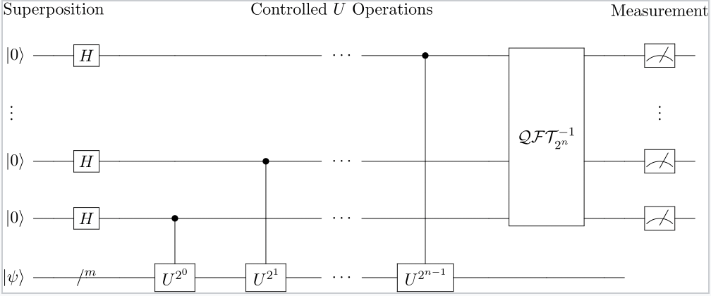
    In order to extract the period, the function is essentially spread in an unobservered superposition across the entire (exponential) set of integers $x$ from $0$ to $2^n-1$, and the exponentials computed via controlled modular exponentiation. Then the iQFT (inverse quantum Fourier transform) is applied to this overall state. The QFT is fast, in that it runs in $O(n\log(n))$ time despite operating on $2^n$ states, since it can operate on tensor products of $n$ qubits. This allows efficient and polynomial time extraction of the period $r$ after a quick classical computation via continued fractions to get the actual factors.

    This algorithm was discovered by Peter W. Shor: “Algorithms for quantum computation: discrete logarithms and factoring”, Presented at the 35th Annual Symposium on Foundations of Computer Science (FOCS) in 1994.


    For elliptic curves, we take a plane curve $E: y^2 = x^3 + Ax + B$ over a finite field $F_p$, whose points form an abelian group. Choose a base point $P$. Alice picks a secret number a, and lets $P_0 = aP$ (add $P$ to itself $a$ times ), her public key. Bob picks a secret number $b$ and computes $P_1 = bP$, his public key. For the key exchange, Alice computes $aP_1 = abP$ and Bob computes $bP_0 = abP$, so they get the same point on the curve, which can be used to derive a shared key. Note that given $(aP, P)$ it is very difficult to determine $a$. This is known as the elliptic curve discrete logarithm problem (ECDLP), and is analogous to RSA where here we are using the addition in the elliptic curve group $E(F_p)$.

    The key sizes for elliptic curves are much smaller than RSA (256 bit ECC ~ 3072 bit RSA).

    A variant of Shor’s algorithm which still performs Fourier sampling just over the abelian group of the elliptic curve $E(F_p)$ rather than the multiplicative group of integers mod $n$. Thus, this is an effective attack on the ECDLP.


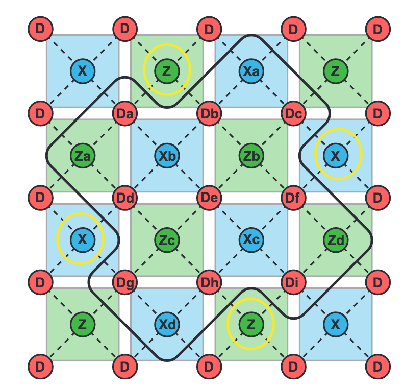
    There is a lot of current discussion re: when quantum computers will become reliable, fault-tolerant, error corrected, and large enough to perform useful computation. Currently there are 127 qubit systems available publicly via IBM. Google also has similar sized machines. The best error correction codes appear to be surface codes, with a $d \times d$ array with $d=7$ qubits, and then hundreds or thousands of physical qubits per logical qubit. This allows the correction of up to 3 errors.

    Surface codes diagram
    Surface codes and logical qubits

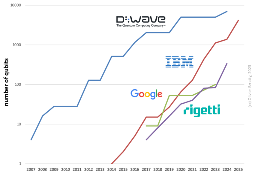
    In general, it may take awhile before there are thousands of qubits required to break something like RSA-1024, which would mean factoring a 1024-bit integer. Estimates range, but something like 5-10 years seems plausible, especially given the exponential nature of progress with respect to number of qubits. To that end, NIST has stated that cryptographic schemes like RSA and ECC with 128 bit security levels will be deprecated by Dec. 31st 2030, and no longer allowed by Dec. 31st 2035. This means that the transition to post-quantum cryptography has already begun, and will probably accelerate over the next five years with many systems being replaced.

    Number of qubits over time
    Number of physical qubits over time

    NIST, Transition to Post-Quantum Cryptography Standards:
    https://csrc.nist.gov/pubs/ir/8547/ipd

    There is a major issue in the meantime that encrypted data that is collected (“harvested”) now will be able to be decrypted later by sufficiently large quantum computers later (“harvest now, decrypt later”). Therefore it is crucial that these systems and databases are replaced as soon as possible.

    To this end, NIST ran a competition to determine the best among a selection of competing post-quantum cryptography standards.

    https://csrc.nist.gov/projects/post-quantum-cryptography/post-quantum-cryptography-standardization

    In the end, the three winners were: CRYSTALS-Dilithium, CRYSTALS-KYBER and SPHINCS+, from which FIPS 203, FIPS 204, and FIPS 205 are respectively derived.

    • Crystals-Dilithium is a digital signature scheme, used for signing and verification. It is based on lattice problems like module-LWE and module-SIS.
    • CRYSTALS-KYBER is a key encapsulation mechanism, used for generating and encrypting a shared symmetric key to be used with another symmetric key encryption scheme. These are based on lattice problems like module-LWE.
    • SPHINCS+ is a stateless hash-based digital signature scheme — meaning it relies purely on hash functions (like SHA-256) for its security, rather than number-theoretic problems or lattices.

    We’ll primarily focus on lattice-based cryptography methods in this post. These are cryptosystems based on algebraic lattices which are very similar to rings of integers in algebraic number fields (like the cyclotomic integers $\mathbb{Z}[x]/(x^n-1)$, but using $x^n+1$ instead, and working over $\mathbb{Z}_q$ rather than $\mathbb{Z}$).

    Each system is based on a computationally hard problem that currently does not have a polynomial time quantum algorithm to solve it. We’ll go into more detail later, but examples of these problems are:

    • Learning with errors (LWE): Given a set of noisy linear equations, find the secret vector. In mathematical terms, you’re given a set of noisy linear combinations of a secret vector, and the task is to recover the secret vector despite the noise.
    • Shortest vector problem (SVP): Given a lattice, find the shortest non-zero vector in that lattice. This is known to be a hard problem in general lattices, and it’s often used as the foundation for other cryptographic protocols. The hardness arises when the given basis is not orthogonal.
    • Closest vector problem (CVP): Given a lattice and a target point, find the closest lattice point to that target. In cryptographic settings, this is used for things like encryption or key exchange protocols.
    • ring-LWE: This is a specialized version of LWE, where the secret and error terms live in a ring structure, which makes the problem more efficient but still computationally hard.
    • module-LWE: Similar to Ring-LWE, but operates in a module setting, which generalizes the ring structure to a rank $k$ module over the ring.

    In this post, we’ll primarily focus on ring-LWE, module-LWE, and FIPS 203.

    FIPS 203 is the module-lattice key encapsulation mechanism (ML-KEM) derived from CRYSTALS-Kyber. It does use module-LWE under the hood in the internal PKE (public key encryption) portion, which we’ll cover in detail later.

    We’ll begin with ring-LWE, a post-quantum fully homomorphic encryption scheme.


    ring-LWE, homomorphic encryption

    For modern cryptography, we aim to find problems that are impractical or ideally impossible to solve, even on a quantum computer.


    The “learning with errors” (LWE) problem, along with its ring-LWE variant, are examples of such problems. It involves distinguishing between two distributions:

    • A set of random linear equations perturbed by a small error (noise)
    • A truly uniform random distribution


    Given $(\bf{A}, \bf{b}) \in \mathbb{Z}_q^{n \times m} \times \mathbb{Z}_q^m$ where $\bf{b} = \bf{A}\bf{s} + \bf{e} \text{ mod } q$:

    • $\bf{A}$ is a known random matrix
    • $\bf{s}$ is a secret vector
    • $\bf{e}$ is a noise vector sampled from a narrow error distribution
    • $q$ is a large modulus


    The goal is to recover the secret $\bf{s}$ or distinguish $(\bf{A},\bf{b})$ from uniformly random samples.

    We’d like to ensure that instances of LWE are hard in the average case. This is done by proving reductions from well-known hard problems in computer science:

    • $\bf{GapSVP}$: Shortest vector problem with a gap
    • $\bf{SIVP}$: Shortest independent vector problem

    These lattice problems are:

    • NP-hard in their exact versions
    • Computationally hard in their approximate versions


    The variant we focus on is ring-LWE, where the lattices are number-theoretic and derived from ideals in certain polynomial rings:

    $R_q = \mathbb{Z}_q[x]/(f(x))$


    where $f(x)$ is typically a polynomial like $x^n – 1$. However, this choice is insecure. Instead, we use:

    $f(x) = x^n+1$

    where $n$ is a power of two. This is the “anti-cyclotomic” ring of integers.

    The hard problem becomes:

    • $\bf{Ideal-SVP}$: Shortest vector problem for ideal lattices

    Consider the ring $R = \mathbb{Z}[x]/(x^n + 1)$:

    • This is a $\mathbb{Z}$-module of rank $n$.
    • Any element $a(x) \in R$ can be written as: $a(x) = \sum_{i=0}^{n-1} c_i x^i$
    • The vector $(c_i)_{i=0}^{n-1}$ is the coefficient vector, making $R \cong \mathbb{Z}^n$.
    • $(x^n + 1)$ is an ideal, and elements $e(x) \in R$ map to elements in this lattice.
    • The error $e(x)$ corresponds to a short vector (in the Euclidean norm) in the lattice, representing a small perturbation.

    Ideal lattices inherit the ring’s structure, such as multiplication by polynomials.


    Solving ring-LWE allows efficient recovery of short vectors in ideal lattices:

    • Ring-LWE enables recovery of the secret $s(x)$, which corresponds to information about the underlying lattice structure.
    • Decoding the noisy lattice point perturbed by $e(x)$ reveals a short vector.

    The reduction shows that solving ring-LWE allows decoding perturbed lattice points for any ideal lattice in $R$, solving Ideal-SVP in the process.


    Our goal is to introduce the simplest possible implementation of the ring-LWE encryption scheme.

    • Choose a moderately large prime $p$ and large $n$ such that n|p-1
    • $n$ should be a power of two and $512$ or above
    • Example: $p = 12289$

    Let $R_p := \mathbb{F}_p[x]/(x^n+1)$.

    This is a finite ring with $p^n$ elements. It is not a finite field, as $x^n+1$ factors modulo $p$ (though it is irreducible over $\mathbb{Z}$).

    The elements look like:


    $$R_p = \{a_{n-1}x^{n-1} + a_{n-2}x^{n-2} + \ldots + a_1x + a_0: a_i \in \mathbb{F}_p\}$$

    Public Setup

    The public setup involves the following:

    • A prime $p$ and dimension $n$ resulting in $R_p$
    • A moderately large integer $k \in \mathbb{Z}$
    • A notion of small, as applied to elements of $R_p$

    These will be “ternary polynomials” with coefficients in ${-1,0,+1}$. The coefficients could also be drawn from a normal distribution centered at $0$ with some standard deviation.

    Key Generation: Private/Public Keypair


    Bob creates a private/public keypair as follows:

    • Bob selects a small random element $s$ of $R_p$
    • Bob selects a small random element $e_1$ of $R_p$
    • Bob defines $(a, b = as + e_1) \in R_p \times R_p$
    • The element $e_1$ can be discarded
    • Bob keeps $s$ as his secret key
    • Bob makes $(a,b)$ public as his public key

    Encryption by Alice


    Alice encrypts a message $m$ as follows:

    • Select a small random $r \in R_p$ (ephemeral key)
    • Select small random $e_2, e_3 \in R_p$
    • Define $v = ar + e_2$, $w = br + e_3 + km$
    • Alice may discard $k$, $e_2$, and $e_3$
    • The ciphertext is $(v, w)$, which is sent to Bob

    Decryption by Bob

    Bob decrypts the message:

    • Compute $x = w – vs$
    • Round $x$ to the nearest multiple of $k$
    • The result should be an integer; divide it by $k$ to reveal the message $m$

    Homomorphic Encryption

    Homomorphic encryption allows computations to be performed on encrypted data without needing to decrypt it first. This enables privacy-preserving computations.

    • Encryption: The data is encrypted using a homomorphic encryption scheme.
    • Computation: Operations such as addition or multiplication are performed directly on the encrypted data.
    • Decryption: The result of the computation is decrypted to reveal the final outcome.

    If $enc(x)$ represents the encryption of data $x$, and $\oplus$ denotes addition on encrypted data, and $\otimes$ represents multiplication on encrypted data:

    • $enc(x + y) = enc(x) \oplus enc(y)$
    • $enc(x \times y) = enc(x) \otimes enc(y)$

    Homomorphic encryption can be used in cloud computing, privacy-preserving machine learning, and secure multi-party computations.

    Code Examples

    code:
    https://crates.io/crates/ring-lwe

    Key generation:

    pub fn keygen(params: &Parameters, seed: Option<u64>) -> ([Polynomial<i64>; 2], Polynomial<i64>) {
    
    //rename parameters
    let (n, q, f, omega) = (params.n, params.q, &params.f, params.omega);
    
    // Generate a public and secret key
    let sk = gen_ternary_poly(n, seed);
    let a = gen_uniform_poly(n, q, seed);
    let e = gen_ternary_poly(n, seed);
    let b = polyadd(&polymul_fast(&polyinv(&a,q), &sk, q, &f, omega), &polyinv(&e,q), q, &f); // b = -a*sk - e
                                            
    // Return public key (b, a) as an array and secret key (sk)
    ([b, a], sk)
    }
    

    We generate the secret key, $a$, $e$ as random polynomials, ensuring $a$ is spread out and uniform whereas $sk$ and $e$ are “small” ternary polynomials. We then compute $b = -a*sk – e$, yielding the public key $[b,a]$ and secret key $sk$.

    Encryption takes in a public key and plaintext polynomial and produces ciphertext:

    
    pub fn encrypt( 
       pk: &[Polynomial<i64>; 2],    // Public key (b, a)
       m: &Polynomial<i64>,        // Plaintext polynomial
       params: &Parameters,       //parameters (n,q,t,f)
       seed: Option<u64>            // Seed for random number generator
    ) -> [Polynomial<i64>; 2] {
       let (n,q,t,f,omega) = (params.n, params.q, params.t, &params.f, params.omega);
       // Scale the plaintext polynomial. use floor(m*q/t) rather than floor (q/t)*m
       let scaled_m = mod_coeffs(m * q / t, q);
    
       // Generate random polynomials
       let e1 = gen_ternary_poly(n, seed);
       let e2 = gen_ternary_poly(n, seed);
       let u = gen_ternary_poly(n, seed);
    
       // Compute ciphertext components
       let ct0 = polyadd(&polyadd(&polymul_fast(&pk[0], &u, q, f, omega), &e1, q, f),&scaled_m,q,f);
       let ct1 = polyadd(&polymul_fast(&pk[1], &u, q, f, omega), &e2, q, f);
    
       [ct0, ct1]
    }


    We scale the plaintext polynomial via $\text{scaled\_m} = \lfloor q/t \rceil m$ and mod coefficients by $q$. Then generate random ternary polynomials $e_1$, $e_2$, $u$. Then $ct_0 = pk[0]*u+e_1+\text{scaled\_m}$ and $ct_1 = pk[1]*u + e_2$, and the final ciphertext is the pair $[ct_0,ct_1]$.

    Finally, decryption:

    
    pub fn decrypt(
        sk: &Polynomial<i64>,    // Secret key
        ct: &[Polynomial<i64>; 2],        // Array of ciphertext polynomials
        params: &Parameters
       ) -> Polynomial<i64> {
       let (_n,q,t,f,omega) = (params.n, params.q, params.t, &params.f, params.omega);
       let scaled\_pt = polyadd(&polymul_fast(&ct[1], sk, q, f, omega),&ct[0], q, f);
       let mut decrypted_coeffs = vec![];
       let mut s;
       for c in scaled_pt.coeffs().iter() {
          s = nearest_int(c*t,q);
          decrypted_coeffs.push(s.rem_euclid(t));
       }
       Polynomial::new(decrypted_coeffs)
    }


    We compute $\text{scaled\_pt} = ct[1]*sk + ct[0]$, then for each coefficient $c$ in $\text{scaled\_pt}$ compute $\lfloor ct/q \rceil$ and take the remainder modulo $t$. The polynomial of coefficients is the decrypted message.

    Keygen/encrypt/decrypt from start to finish:

            
    let seed = None; //set the random seed
    let message = String::from("hello");
    let params = Parameters::default();
    let keypair = keygen_string(&params,seed);
    let pk_string = keypair.get("public").unwrap();
    let sk_string = keypair.get("secret").unwrap();
    let ciphertext_string = encrypt_string(&pk_string, &message, &params,seed);
    let decrypted_message = decrypt_string(&sk_string, &ciphertext_string, &params);
    assert_eq!(message, decrypted_message, "test failed: {} != {}", message, decrypted_message);


    We use serialization and base64 encoding to compress the output strings.

    For the homomorphic encryption, we only achieve a single product, so this is “leveled homomorphic encryption” at level one for the time being. We use a form of relinearization described here:

    https://crypto.stackexchange.com/questions/113740/how-to-correctly-multiply-homomorphically-two-rlwe-based-encrypted-numbers/113741

    We perform multiplications of the ciphertext polynomials and the divide by $\Delta = q/t$. The implementation is as follows:

    
    let seed = None; //set the random seed
    let mut params = Parameters::default();
    let (q, t, f) = (params.q, params.t, &params.f);
    params.q = q*q;
    params.omega = omega(params.q, 2*params.n);
    
    //create polynomials from ints
    let m0_poly = Polynomial::new(vec![1, 0, 1]);
    let m1_poly = Polynomial::new(vec![0, 0, 1]);
    
    // Generate the keypair
    let (pk, sk) = keygen(&params,seed);
    
    // Encrypt plaintext messages
    let u = encrypt(&pk, &m0_poly, &params, seed);
    let v = encrypt(&pk, &m1_poly, &params, seed);
    
    let plaintext_prod = polymul(&m0_poly, &m1_poly, t, &f);
    
    //compute product of encrypted data, using non-standard multiplication
    let c0 = polymul(&u[0],&v[0],params.q,&f);
    let u0v1 = &polymul(&u[0],&v[1],params.q,&f);
    let u1v0 = &polymul(&u[1],&v[0],params.q,&f);
    let c1 = polyadd(u0v1,u1v0,params.q,&f);
    let c2 = polymul(&u[1],&v[1],params.q,&f);
    
    //compute c0 + c1*s + c2*s*s
    let c1_sk = &polymul(&c1,&sk,params.q,&f);
    let c2_sk_squared = &polymul(&polymul(&c2,&sk,params.q,&f),&sk,params.q,&f);
    let ciphertext_prod = polyadd(&polyadd(&c0,c1_sk,params.q,&f),c2_sk_squared,params.q,&f);
    //let delta = q / t, divide coeffs by 1 / delta^2
    let delta = q / t;
    let decrypted_prod = mod_coeffs(Polynomial::new(ciphertext_prod.coeffs().iter().map(|&coeff| nearest_int(coeff,delta * delta) ).collect::<Vec<_>>()),t);
                                                
    assert_eq!(plaintext_prod, decrypted_prod, "test failed: {} != {}", plaintext_prod, decrypted_prod);


    We’d eventually like to improve this to be fully homomorphic encryption.


    module-lwe

    While the polynomial ring structure of ring-LWE is rich and useful for things like homomorphic encryption (since they’re based on rings, the structure is readily available), this additional algebraic structure is thought to make this system potentially vulnerable to attacks that exploit these number theoretic aspects.

    There is a generalization of of ring-LWE called module-LWE which uses the rank $k$ free module $R_q^k$ instead of just the ring $R_q$ (when $k=1$), where again $R_q = \mathbb{Z}_q/(x^n+1)$ as in ring-LWE. The elements of $R_q^k$ are k-tuples of polynomials in $R_q$.

    Module-LWE works sort of like a hybrid between the original LWE scheme and ring-LWE, combining both matrix operations and polynomial multiplication.

    Advantages of module-LWE:

    • Scalability: The main way to increase the security of ring-LWE is to increase the polynomial modulus degree $n$, but since this is alwayts a power of two there is no way to make a small increase in security if you are close to the necessary threshold. On the other hand, in module-LWE you can also increase the module rank $k$, which can be any nonnegative integer.
    • Parallelization: Many of the computations in module-LWE involve matrix operations, which can be easily parallelized.
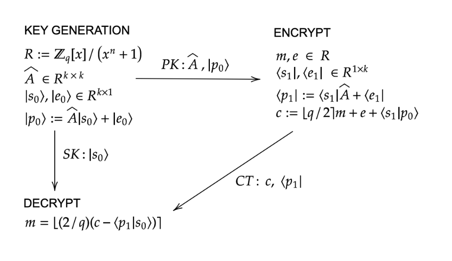
    module-lwe diagram for keygen, encrypt, ecrypt
    module-lwe diagram for keygen, encrypt, decrypt

    Public Setup

    The public setup involves the following:

    • A prime $q$ and modulus degree $n$ resulting in the ring $R_q$
    • Module rank $k$
    • A notion of “small”, as applied to elements of $R_q^k$

      • These are $k$-tuples of ternary polynomials, with coefficients in $\{-1,0,+1\}$

    Key Generation

    Bob selects a private/public keypair as follows:

    • Bob selects a small random element $|s_0 \rangle$ of $R_q^{k+1}$
    • Bob selects a small random element $|e_0 \rangle$ of $R_q^{k+1}$
    • Bob selects a uniformly random matrix $\hat{A}$ in $R_q^{k \times k}$
    • Bob defines $|p_0 \rangle := \hat{A}|s_0 \rangle + |e_0 \rangle$

    The element $|e_0 \rangle$ can be discarded.

    • Bob keeps $|s_0$ as his secret key
    • Bob makes $(\hat{A},|p_0\rangle)$ public as his public key

    Encryption by Alice

    Alice encrypts a message $m \in \mathbb{Z}_2[x]/(x^n+1)$ as follows:

    • Alice selects a small random element $\langle s_1 |$ of $R_q^{1 \times k}$ (ephemeral key)
    • Alice selects small random $\langle e_1 | \in R_q^{1 \times k}$ and $e \in R_q$
    • Alice defines $\langle p_1 | := \langle s_1 | \hat{A} + \langle e_1 |$ and $c := \lfloor q/2 \rceil m + e + \langle s_1 | p_0 \rangle$

    Alice may discard $\langle s_1 |$, $\langle e_1 |$, and $e$

    • The ciphertext is $(c, \langle p_1 |)$, which is sent to Bob

    Decryption by Bob

    Bob decrypts the message as follows:

    • Compute $x = c – \langle p_1 | s_0 \rangle$
    • Divide by $\lfloor q/2 \rceil$
    • Round the coefficients to the nearest integer modulo $2$
    • the result is the message $m$

    Correctness

    $x = c – \langle p_1 | s_0 \rangle$

    $= (\lfloor q/2 \rceil m + e + \langle s_1 | p_0 \rangle ) – (\langle s_1 | \hat{A} + \langle e_1 |)|s_0 \rangle$

    $= \lfloor q/2 \rceil m + e + \langle s_1 | \hat{A} | s_0 \rangle + \langle s_1 | e_0 \rangle – \langle s_1 | \hat{A} | s_0 \rangle + \langle e_1 | s_0 \rangle$

    $= \lfloor q/2 \rceil m + \text{small polynomials}$

    so dividing by $\lfloor q/2 \rceil$ and rounding coefficients to the nearest integer modulo $2$ returns $m$.

    Code Examples

    We’ve published our Rust implementation as a crate at https://crates.io/crates/module-lwe.

    The key generation is fairly straightforward:

    
    pub fn keygen(
        params: &Parameters,
        seed: Option<u64> //random seed
    ) -> ((Vec<Vec<Polynomial<i64>>>, Vec<Polynomial<i64>>), Vec<Polynomial<i64>>) {
        let (n,q,k,f,omega) = (params.n, params.q, params.k, &params.f, params.omega);
        //Generate a public and secret key
        let a = gen_uniform_matrix(n, k, q, seed);
        let sk = gen_small_vector(n, k, seed);
        let e = gen_small_vector(n, k, seed);
        let t = add_vec(&mul_mat_vec_simple(&a, &sk, q, &f, omega), &e, q, &f);
        
        //Return public key (a, t) and secret key (sk) as a 2-tuple
        ((a, t), sk)
    }


    We essentially generate a uniformly random matrix with coefficients in $R_q$, generate the secret key and small error vector, compute $t$, and this gives the public and private keys.

    Encryption is also rather brief:

    
    pub fn encrypt(
        a: &Vec<Vec<Polynomial<i64>>>,
        t: &Vec<Polynomial<i64>>,
        m_b: &Vec<i64>,
        params: &Parameters,
        seed: Option<u64>
    ) -> (Vec<Polynomial<i64>>, Polynomial<i64>) {
    
        //get parameters
        let (n, q, k, f, omega) = (params.n, params.q, params.k, &params.f, params.omega);
        
        //generate random ephermal keys
        let r = gen_small_vector(n, k, seed);
        let e1 = gen_small_vector(n, k, seed);
        let e2 = gen_small_vector(n, 1, seed)[0].clone(); // Single polynomial
    
        //compute nearest integer to q/2
        let half_q = nearest_int(q,2);
    
        // Convert binary message to polynomial
        let m = Polynomial::new(vec![half_q])*Polynomial::new(m_b.to_vec());
    
        // Compute u = a^T * r + e_1 mod q
        let u = add_vec(&mul_mat_vec_simple(&transpose(a), &r, q, f, omega), &e1, q, f);
    
        // Compute v = t * r + e_2 - m mod q
        let v = polysub(&polyadd(&mul_vec_simple(t, &r, q, &f, omega), &e2, q, f), &m, q, f);
    
        (u, v)
    }


    We generate random ephemeral keys as small error vectors again with coefficients in $R_q$, compute $\lfloor q/2 \rceil$, convert the binary message to a polynomial with $\{0,1\}$ coefficients, then compute the vector $u$ and polynomial $v$. The ciphertext is $(u,v)$.

    Finally, decrypt gives the plaintext message given the ciphertext and secret keys:

    
    pub fn decrypt(
        sk: &Vec<Polynomial<i64>>,    //secret key
        u: &Vec<Polynomial<i64>>, //ciphertext vector
        v: &Polynomial<i64> ,		//ciphertext polynomial
        params: &Parameters
    ) -> Vec<i64> {
        let (q, f, omega) = (params.q, &params.f, params.omega); //get parameters
        let scaled_pt = polysub(&v, &mul_vec_simple(&sk, &u, q, &f, omega), q, f); //Compute v-sk*u mod q
        let half_q = nearest_int(q,2); // compute nearest integer to q/2
        let mut decrypted_coeffs = vec![];
        let mut s;
        for c in scaled_pt.coeffs().iter() {
            s = nearest_int(*c,half_q).rem_euclid(2);
            decrypted_coeffs.push(s);
        }
        decrypted_coeffs
    }


    We compute $v – sk*u$, a polynomial, then again compute $\lfloor q/2 \rceil$, and then compute $c / \lfloor q/2 \rceil \text{ mod } 2$ for each coefficient $c$. This yields the decrypted message.

    Note that module-lwe is not fully homomorphic, but it is additively homomorphic.

      
    let seed = None; //set the random seed
    let params = Parameters::default();
    let (n, q, f) = (params.n, params.q, &params.f);
    
    let mut m0 = vec![1, 0, 1];
    m0.resize(n, 0);
    let mut m1 = vec![0, 0, 1];
    m1.resize(n, 0);
    let mut plaintext_sum = vec![1, 0, 0];
    plaintext_sum.resize(n, 0);
    let (pk, sk) = keygen(&params,seed);
    
    // Encrypt plaintext messages
    let u = encrypt(&pk.0, &pk.1, &m0, &params, seed);
    let v = encrypt(&pk.0, &pk.1, &m1, &params, seed);
    
    // Compute sum of encrypted data
    let ciphertext_sum = (add_vec(&u.0,&v.0,q,f), polyadd(&u.1,&v.1,q,f));
    
    // Decrypt ciphertext sum u+v
    let mut decrypted_sum = decrypt(&sk, &ciphertext_sum.0, &ciphertext_sum.1, &params);
    decrypted_sum.resize(n, 0);
    
    assert_eq!(decrypted_sum, plaintext_sum, "test failed: {:?} != {:?}", decrypted_sum, plaintext_sum);


    That is, if we encrypt $u$, $v$ to get $enc(u)$ and $enc(v)$, then form the sum $enc(u)+enc(v)$, we have $dec(enc(u)+enc(v)) = u+v$, so we recover the original sum.

    We use a serialization and base64 encoding on the resulting arrays of ints to store the keys in a compact form.

    Here is the entire encryption process from start to finish:

      
    let seed = None; //set random seed
    let message = String::from("hello");
    let params = Parameters::default();
    let keypair = keygen_string(&params,seed);
    let pk_string = keypair.get("public").unwrap();
    let sk_string = keypair.get("secret").unwrap();
    let ciphertext_string = encrypt_string(&pk_string, &message, &params,seed);
    let decrypted_message = decrypt_string(&sk_string, &ciphertext_string, &params);
    assert_eq!(message, decrypted_message, "test failed: {} != {}", message, decrypted_message);


    Note here we use the string methods which generate the keys, ciphertext, and message as a string.


    the number theoretic transform (NTT)

    https://crates.io/crates/ntt

    In both of the above schemes, we perform a certain number of polynomial multiplications. There is a way to significantly speed this operation up from $\mathcal{O}(n^2)$ to $\mathcal{O}(n\log(n))$.

    Polynomials have the property that their multiplication can be viewed as a cyclic convolution of the coefficients. That is, polynomial multiplication is just $f \star g$.

    In general, the Fourier transform will take a convolution of functions to a pointwise product, so that $\mathcal{F}(f \star g) = \mathcal{F}(f) \cdot \mathcal{F}(g)$.

    We can then perform multiplication in the original domain by performing an inverse Fourier transform, that is:

    $f \star g = \mathcal{F}^{-1}(\mathcal{F}(f) \cdot \mathcal{F}(g))$

    Since we are working over the discrete ring $\mathbb{Z}_q[x]/(x^n+1)$, we instead use a version of the NTT which is exact and takes arrays of integers to arrays of integers. This is called the “number theoretic transform”, and relies on a root of unity in the given coefficient ring.

    In $\mathbb{Z}_q$, the roots of unity are given by examining the multiplicative group $(\mathbb{Z}_q)^{\times}$, which is just a cyclic group of order $q-1$ if $q$ is prime. Generally, the size of the group is $\varphi(q)$, the Euler totient function, and will have cyclic factors of size $\varphi(p_i^{k_i})$ for each prime factor $p_i$ of $q$. It is only cyclic when $q=2, 4, p^k, 2p^k$ which is the case we’ll focus on, in particular $p^k$.

    Thus, to find an $n^{th}$ root of unity, we need that $n \mid \varphi(q)$. If we then have a primitive root of unity $g$, an element which generates the entire multiplicative group $(\mathbb{Z}_q)^{\times}$, then $\omega = g^{\varphi(q)/n}$ will be an $n^{th}$ root of unity. Again, $\omega$ is just an integer modulo $q$.

    The NTT is then just:

    $\hat{a}_k = \sum_{j=0}^{n-1} a_j \omega^{jk} \text{ mod } q \quad \text{for } k=0, \ldots, n-1$

    One can think of this as the discrete Fourier transform with a different root of unity. This operation can be represented by a matrix.

    In order to optimize this operation, we use the Cooley–Tukey method which uses butterfly operations recursively split the arrays in half. This is a reason that $n$ must be a power of $2$.

    
    pub fn ntt(a: &[i64], omega: i64, n: usize, p: i64) -> Vec<i64> {
    let mut result = a.to_vec();
    let mut step = n/2;
    while step > 0 {
        let w_i  = mod_exp(omega, (n/(2*step)).try_into().unwrap(), p);
        for i in (0..n).step_by(2*step) { 
            let mut w = 1;
            for j in 0..step {
                let u = result[i+j];
                let v = result[i+j+step];
                result[i+j] = mod_add(u,v,p);
                result[i+j+step] = mod_mul(mod_add(u,p-v,p),w,p);
                w = mod_mul(w,w_i,p);
            }
        }
        step/=2;
    }
    result
    }


    n.b. If one needs an $n^{th}$ root of unity $\text{mod } N$ and $N$ is composite, It’s possible to find an $n^{th}$ root of unity $\omega_i$ for each cyclic factor of size $\varphi(p_i^{k_i})$ as long as $n \mid \varphi(p_i^{k_i})$ for each $i$. Then one can use the Chinese remainder theorem isomorphism to pull back each $\omega_i$ to get a root of unity $\omega$ which satisfies the necessary properties, namely $\sum_{j=0}^{n-1} \omega^{jk} = 0$ for $1 \le k < n$.


    module-lattice key encapsulation mechanism (ML-KEM), FIPS 203, Kyber

    code:
    https://crates.io/crates/mlkem-fips203

    FIPS 203 paper:
    https://nvlpubs.nist.gov/nistpubs/FIPS/NIST.FIPS.203.pdf

    Kyber paper:
    https://eprint.iacr.org/2017/634.pdf

    While both ring-LWE and module-LWE represent post-quantum, lattice-based cryptosystems, neither of them have been directly standardized yet. Ring-LWE is more useful for homomorphic encryption, with the potential future security vulnerabilities arising from the direct algebraic ring structure. Module-LWE is more useful as an internal component of what is called a key encapsulation mechanism, which is a way to generate a shared key K, and encrypt the key itself to get a ciphertext version cwhich can be transmitted over an insecure channel. This is meant to be used in conjunction with another symmetric key cryptosystem, for instance AES which was standardized by NIST in FIPS PUB 197 on Nov. 26, 2001.

    For our implementation, we initially made use of our module-lwe implementation but then decided to follow closely Giacomo Pope’s implementation in Python, kyber-py:

    https://github.com/giacomopope/kyber-py

    The end goal will be to create the key encapsulation mechanism, which generates a public key pk and secret key sk, encapsulates pkto get the shared key K and ciphertext c, then use the secret key sk to decapsulate c to obtain the shared key K.

    We need to be careful about how we generate randomness. We use a DRBG (deterministic random bit generator) to generate a stream of random bytes if the seed is set, and otherwise use OS/system randomness via getrandom.

    
    use aes_ctr_drbg::DrbgCtx;
    
    ...    
    
    /// Set the DRBG to be used for random bytes
        pub fn set_drbg_seed(&mut self, seed: Vec<u8>) {
            let p = vec![48, 0]; // personalization string must be min. 48 bytes long
            let mut drbg = DrbgCtx::new(); // instantiate the DRBG
            drbg.init(&seed, p); // initialize the DRBG with the seed
            self.drbg = Some(drbg); // Store the DRBG in the struct
        }
    
    ...
    
    fn gen_random_bytes(size: usize, drbg: Option<&mut DrbgCtx>) -> Vec<u8> {
        let mut out = vec![0; size];
        if let Some(drbg) = drbg {
            drbg.get_random(&mut out);
        }
        else {
            getrandom(&mut out).expect("Failed to get random bytes");
        }
        out
    }


    We use two psuedorandom functions, prf_2 and prf_3, one for each value of eta=2 or eta=3, where the size of Shake256 hash is either 128 or 192 bytes, respectively.

    
    pub fn prf_2(s: Vec<u8>, b: u8) -> Vec<u8> {
        // Concatenate s and b
        let mut m = s;
        m.push(b);
        // Apply shake_256 hash
        let mut shake_256hasher = Shake256Hasher::<128>::default();
        shake_256hasher.write(&m);
        let bytes_result = HasherContext::finish(&mut shake_256hasher);
        bytes_result[0..].to_vec()
    }
    
    pub fn prf_3(s: Vec<u8>, b: u8) -> Vec<u8> {
        // Concatenate s and b
        let mut m = s;
        m.push(b);
        // Apply shake_256 hash
        let mut shake_256hasher = Shake256Hasher::<192>::default();
        shake_256hasher.write(&m);
        let bytes_result = HasherContext::finish(&mut shake_256hasher);
        bytes_result[0..].to_vec()
    }


    eta is a parameter related to the width of a CBD (centered binomial distribution), which is given as follows:

    $X = \sum_{i=1}^{\eta} (a_i – b_i), \quad \text{where } a_i, b_i \sim \text{Ber}(1/2)$

    This allows us to generate random polynomials.

    
    pub fn cbd(input_bytes: Vec<u8>, eta: usize, n:usize) -> Polynomial<i64> {
        assert_eq!(eta*n/4, input_bytes.len(), "input length must be eta*n/4");
        let mut coefficients = vec![0;n];
        let mut t = BigUint::from_bytes_le(&input_bytes);
        let mask = BigUint::from((1 << eta)-1 as u64);
        let mask2 = BigUint::from((1 << 2*eta)-1 as u64);
        for i in 0..n {
            let x = t.clone() & mask2.clone();
            let a = (x.clone() & mask.clone()).count_ones() as i64;
            let b = ((x.clone() >> eta) & mask.clone()).count_ones() as i64;
            t >>= 2*eta;
            coefficients[i] = a-b;
        }
        Polynomial::new(coefficients)
    }


    We also use an extendable output function (XOF) to extend a random 32 byte input given two domain separation parameters to get an 840 byte random output:

    
    pub fn xof(bytes32: Vec<u8>, i: u8, j: u8) -> Vec<u8> {
        // Concatenate bytes32, i, and j
        let mut m = bytes32;
        m.push(i);
        m.push(j);
        // Apply shake_128 hash
        let mut shake_128hasher = Shake128Hasher::<840>::default();
        shake_128hasher.write(&m);
        let bytes_result = HasherContext::finish(&mut shake_128hasher);
        bytes_result[0..].to_vec()
    }


    This is used to generate a random matrix from a seed. Note this is essentially the matrix from module-lwe, and is a random k x k matrix whose coefficients are polynomials in the ring $R_q$. In this case, we are setting q=3329 as a global parameter, a prime, noting that $\mathbb{Z}_q$ is a field.

    
    pub fn generate_matrix_from_seed(
        rho: Vec<u8>,
        rank: usize,
        n: usize,
        transpose: bool,
    ) -> Vec<Vec<Polynomial<i64>>> {
        let mut a_data = vec![vec![Polynomial::new(vec![]); rank]; rank];
    
        for i in 0..rank {
            for j in 0..rank {
                let xof_bytes = xof(rho.clone(), j as u8, i as u8);
                a_data[i][j] = Polynomial::new(ntt_sample(xof_bytes, n));
            }
        }
    
        if transpose {
            matrix_transpose(a_data)
        } else {
            a_data
        }
    }


    Note that again we are using the Polynomial<i64> type because it is convenient, but it would make a lot of sense to implement this as a struct with the methods we need for polyadd, polysub, etc. We instead just opt to keep everything as utility functions for now.

    We can use the prf functions to generate an error vector as well:

    
    pub fn generate_error_vector(
        sigma: Vec<u8>,
        eta: usize,
        b: u8,
        k: usize,
        poly_size: usize,
    ) -> (Vec<Polynomial<i64>>, u8) {
        let mut elements = vec![Polynomial::new(vec![]); k];
        let mut current_b = b;
    
        for i in 0..k {
            let prf_output: Vec<u8>;
            if eta == 2 {
                prf_output = prf_2(sigma.clone(), current_b);
            } else if eta == 3 {
                prf_output = prf_3(sigma.clone(), current_b);
            } else {
                panic!("eta must be 2 or 3"); // Handle invalid eta values
            }
            assert_eq!(eta*poly_size/4, prf_output.len(), "eta*poly_size/4 must be 128 or 192 (prf output length)");
            elements[i] = cbd(prf_output, eta, poly_size);
            current_b += 1;
        }
    
        (elements, current_b)
    }


    Similarly we can generate a random polynomial using the cbd function:

    
    pub fn generate_polynomial(
        sigma: Vec<u8>,
        eta: usize,
        b: u8,
        poly_size: usize,
        q: Option<i64>,
    ) -> (Polynomial<i64>, u8) {
        // get the prf_output depending on eta = 2, or eta = 3
        let prf_output: Vec<u8>;
        if eta == 2 {
            prf_output = prf_2(sigma, b);
        } else if eta == 3 {
            prf_output = prf_3(sigma, b);
        } else {
            panic!("eta must be 2 or 3"); // Handle invalid eta values
        }
        let poly = cbd(prf_output, eta, poly_size); // form the polynomial array from a centered binomial dist.
        //if a modulus is set, place coeffs in [0,q-1]
        if let Some(q) = q {
            return (mod_coeffs(poly,q), b + 1);
        }
        (poly, b + 1)
    }


    Now that we’re able to generate random polynomials, error vectors, and matrices, we want to be able to compress/encode and decompress/decode our inputs and outputs.

    To compress a polynomial, we compress its coefficients using this function:

        fn compress_ele(x: i64, d: usize) -> i64 {
            let t = 1 << d;
            let y = (t * x.rem_euclid(3329) + 1664) / 3329; // n.b. 1664 = 3329 / 2
            y % t
        }
    

    To encode a polynomial, we use a bit-width parameter
    d
    which is usually 12 or 1:

    
    pub fn encode_poly(poly: Polynomial<i64>, d: usize) -> Vec<u8> {
    let poly_mod = mod_coeffs(poly.clone(), 3329);
    let mut t = BigUint::zero(); // Start with a BigUint initialized to zero
    let mut coeffs = poly_mod.coeffs().to_vec(); // get the coefficients of the polynomial
    coeffs.resize(256, 0); // ensure they're the right size
    
    for i in 0..255 {
        // OR the current coefficient then left shift by d bits
        t |= BigUint::from(coeffs[256 - i - 1] as u64); // Use BigUint for coefficients
        t <<= d; // Equivalent to t = t * 2^d
    }
    
    // Add the last coefficient
    t |= BigUint::from(coeffs[0] as u64);
    
    // Convert BigUint to a byte vector
    let byte_len = 32 * d;
    let mut result = t.to_bytes_le(); // Convert to little-endian bytes
    result.resize(byte_len, 0); // Ensure the result is exactly `32 * d` bytes
    
    result
    }


    Decode and decompress invert this. For vectors of polynomials, we just compress each polynomial, encode each polynomial, and extend the array of bytes.

    The final important step before describing the actual PKE and encapsulation algorithms is the NTT. Above, we saw that the NTT depended on an $n^{th}$ root of unity. In this case, the other global Kyber parameter is n=256, which is the degree of the polynomials. Since $q=3329$, and since Cooley-Tukey requires a $2n^{th}$ root of unity (a square root of an $n^{th}$ root of unity), this would mean a $512^{th}$ root of unity, which doesn’t exist in $\mathbb{Z}_q$ since $512 \nmid 3328$. Therefore we need to do something different.

    Indeed, the FIPS 203 paper outlines on pg. 24 how to perform an NTT despite this limitation. It uses the Chinese remainder theorem to write the ring $R_q = \mathbb{Z}_q[x]/(x^{256}+1)$ as

    $T_q = \bigoplus_{i=0}^{127}\mathbb{Z}_q[x]/(x^2 – \zeta^{BitRev_7(i)+1})$

    which is a sum of $128$ quadratic terms. This isomorphism means we only need a $256^{th}$ root of unity, which we do have. We just need to compute the bit reversal function, and the $\zeta$’s:

    
    pub fn bit_reverse(i: i64, k: usize) -> i64 {
        let mut reversed = 0;
        let mut n = i;
        
        for _ in 0..k {
            reversed = (reversed << 1) | (n & 1);
            n >>= 1;
        }
    
        reversed
    }
    
    ...
    
    let zetas: Vec<i64> = (0..128)
        .map(|i| mod_exp(17, bit_reverse(i, 7), 3329))
        .collect();


    Here mod_exp is just the modular exponentiation modulo q.

    The NTT is similar to the usual butterfly operations, but we pair coefficients:

        pub fn poly_ntt(poly: Polynomial<i64>, zetas: Vec<i64>) -> Polynomial<i64> {
            let mut coeffs = poly.coeffs().to_vec(); // Convert slice to Vec<i64>
            coeffs.resize(256, 0); // Ensure uniform length
            let mut k = 1;
            let mut l = 128;
            while l >= 2 {
                let mut start = 0;
                while start < 256 {
                    let zeta = zetas[k];
                    k += 1;
                    for j in start..start+l {
                        let t = zeta*coeffs[j+l];
                        coeffs[j+l] = (coeffs[j]-t).rem_euclid(3329);
                        coeffs[j] = (coeffs[j]+t).rem_euclid(3329);
                    }
                    start += 2*l;
                }
                l >>= 1;
            }
            Polynomial::new(coeffs)
        }
    

    With this NTT (and its associated inverse), we can define the ntt for vectors as well by just operating on each coefficient. Since we will deal with polynomials and vectors in their NTT form, we multiply them pointwise, and so we need to carefully define the multiplication in $T_q$:

    
    pub fn ntt_base_multiplication(a0:i64 , a1:i64, b0:i64, b1:i64, zeta:i64) -> (i64, i64) {
        let r0 = (a0*b0+zeta*a1*b1).rem_euclid(3329);
        let r1 = (a1*b0+a0*b1).rem_euclid(3329);
        (r0, r1)
    }
    
    pub fn ntt_coefficient_multiplication(f_coeffs: Vec<i64>, g_coeffs: Vec<i64>, zetas: Vec<i64>) -> Vec<i64> {
        let mut new_coeffs = vec![];
        // Multiply in each of the 128 Z_q[x]/(x^2-zeta) factors
        for i in 0..64 {
            let (r0,r1) = ntt_base_multiplication(
                f_coeffs[4*i+0],
                f_coeffs[4*i+1],
                g_coeffs[4*i+0],
                g_coeffs[4*i+1],
                zetas[64+i]);
            let (r2,r3) = ntt_base_multiplication(
                f_coeffs[4*i+2],
                f_coeffs[4*i+3],
                g_coeffs[4*i+2],
                g_coeffs[4*i+3],
                -zetas[64+i]);
            new_coeffs.append(&mut vec![r0,r1,r2,r3]);
        }
        new_coeffs
    }


    With those definitions, we can define a dot product of vectors using this NTT multiplication:

    
    pub fn mul_vec_simple(v0: Vec<Polynomial<i64>>, v1: Vec<Polynomial<i64>>, q: i64, f: Polynomial<i64>, zetas: Vec<i64>) -> Polynomial<i64> {
        assert!(v0.len() == v1.len());
        let mut result = Polynomial::new(vec![]);
        for i in 0..v0.len() {
            let v0_v1_mult = ntt_multiplication(v0[i].clone(), v1[i].clone(), zetas.clone());
            result = polyadd(result, v0_v1_mult.clone(), q, f.clone());
        }
        mod_coeffs(result, q)
    }


    This allows us to then define multiplication of a matrix times a vector. Now we are ready to define the PKE and encapsulation operations.

    We use different sets of parameters for different levels of security.

    • MLKEM512 (~128 bit security): k=2, eta_1=3, eta_2=2, du=10, dv=4
    • MLKEM768 (~192 bit security): k=3, eta_1=2, eta_2=2, du=10, dv=4
    • MLKEM1024 (~256 bit security): k=4, eta_1=2, eta_2=2, du=11, dv=5

    We keep these in parameters::Parameters.

    The PKE keygen follows Algorithm 13 of FIPS 203:

        
    pub fn _k_pke_keygen(
        &self,
        d: Vec<u8>,
    ) -> (Vec<u8>, Vec<u8>) {
        // Expand 32 + 1 bytes to two 32-byte seeds.
        // Note: rho, sigma are generated using hash_g
        let (rho, sigma) = hash_g([d.clone(), vec![self.params.k as u8]].concat());
    
        // Generate A_hat from seed rho
        let a_hat = generate_matrix_from_seed(rho.clone(), self.params.k, self.params.n, false);
    
        // Set counter for PRF
        let prf_count = 0;
    
        // Generate the error vectors s and e
        let (s, _prf_count) = generate_error_vector(sigma.clone(), self.params.eta_1, prf_count, self.params.k, self.params.n);
        let (e, _prf_count) = generate_error_vector(sigma.clone(), self.params.eta_1, prf_count, self.params.k, self.params.n);
    
        // the NTT of s as an element of a rank k module over the polynomial ring
        let s_hat = vec_ntt(s, self.params.zetas.clone());
        // the NTT of e as an element of a rank k module over the polynomial ring
        let e_hat = vec_ntt(e, self.params.zetas.clone());
        // A_hat @ s_hat + e_hat
        let a_hat_s_hat = mul_mat_vec_simple(a_hat, s_hat.clone(), self.params.q, self.params.f.clone(), self.params.zetas.clone());
        let t_hat = add_vec(a_hat_s_hat, e_hat, self.params.q, self.params.f.clone());
    
        // Encode the keys
        let mut ek_pke = encode_vector(t_hat, 12); // Encoding vec of polynomials to bytes
        ek_pke.extend(rho); // append rho, output of hash function
        let dk_pke = encode_vector(s_hat, 12); // Encoding s_hat for dk_pke
    
        (ek_pke, dk_pke)
    }


    Note that this essentially computes $\hat{t}=\hat{A}\hat{s} + \hat{e}$ and encodes this vector to get the public key, and then just encodes $\hat{s}$ to get the private key.

    Next, the PKE encryption:

        
    pub fn _k_pke_encrypt(
        &self,
        ek_pke: Vec<u8>,
        m: Vec<u8>,
        r: Vec<u8>,
    ) -> Result<Vec<u8>, String> {
    
        let expected_len = ek_pke.len();
        let received_len = 384 * self.params.k + 32;
    
        if expected_len != received_len {
            return Err(format!(
                "Type check failed: ek_pke length mismatch (expected {}, got {})",
                received_len, expected_len
            ));
        }
    
        // Unpack ek
        let (t_hat_bytes_slice, rho_slice) = ek_pke.split_at(ek_pke.len() - 32);
        let t_hat_bytes = t_hat_bytes_slice.to_vec();
        let rho = rho_slice.to_vec();
    
        // decode the vector of polynomials from bytes
        let t_hat = decode_vector(t_hat_bytes.clone(), self.params.k, 12);
    
        // check that t_hat has been canonically encoded
        if encode_vector(t_hat.clone(),12) != t_hat_bytes {
            return Err("Modulus check failed: t_hat does not encode correctly".to_string());
        }
    
        // Generate A_hat^T from seed rho
        let a_hat_t = generate_matrix_from_seed(rho.clone(), self.params.k, self.params.n, true);
    
        // generate error vectors y, e1 and error polynomial e2
        let prf_count = 0;
        let (y, _prf_count) = generate_error_vector(r.clone(), self.params.eta_1, prf_count, self.params.k, self.params.n);
        let (e1, _prf_count) = generate_error_vector(r.clone(), self.params.eta_2, prf_count, self.params.k, self.params.n);
        let (e2, _prf_count) = generate_polynomial(r.clone(), self.params.eta_2, prf_count, self.params.n, None);
    
        // compute the NTT of the error vector y
        let y_hat = vec_ntt(y, self.params.zetas.clone());
    
        // compute u = intt(a_hat.T * y_hat) + e1
        let a_hat_t_y_hat = mul_mat_vec_simple(a_hat_t, y_hat.clone(), self.params.q, self.params.f.clone(), self.params.zetas.clone());
        let a_hat_t_y_hat_intt = vec_intt(a_hat_t_y_hat, self.params.zetas.clone());
        let u = add_vec(a_hat_t_y_hat_intt, e1, self.params.q, self.params.f.clone());
    
        //decode the polynomial mu from the bytes m
        let mu = decompress_poly(decode_poly(m, 1),1);
    
        //compute v = intt(t_hat.y_hat) + e2 + mu
        let t_hat_dot_y_hat = mul_vec_simple(t_hat, y_hat, self.params.q, self.params.f.clone(), self.params.zetas.clone());
        let t_hat_dot_y_hat_intt = poly_intt(t_hat_dot_y_hat, self.params.zetas.clone());
        let t_hat_dot_y_hat_intt_plus_e2 = polyadd(t_hat_dot_y_hat_intt.clone(), e2.clone(), self.params.q, self.params.f.clone());
        let v = polyadd(t_hat_dot_y_hat_intt_plus_e2, mu, self.params.q, self.params.f.clone());
    
        // compress vec u, poly v by compressing coeffs, then encode to bytes using params du, dv
        let c1 = encode_vector(compress_vec(u,self.params.du),self.params.du);
        let c2 = encode_poly(compress_poly(v,self.params.dv),self.params.dv);
    
        //return c1 + c2, the concatenation of two encoded polynomials
        Ok([c1, c2].concat())
    
    }


    We unpack $\hat{t}$ (and check correctness), then generate $\hat{A}^{T}$, generate error vectors $y$, $e_1$, and error polynomial $e_2$. Then we compute $\hat{y}$ (the NTT), and $u = intt(\hat{A}^T*\hat{y}) + e_1$ (a vector). We decode the message $m$ as $\mu$, then compute $v = intt(\hat{t}\cdot\hat{y}) + e_2 + \mu$ (a polynomials). We then compress vector $u$ and polynomial $v$ to get the ciphertext $c_1$, $c_2$.

    Decryption is as follows:

        
    pub fn _k_pke_decrypt(&self, dk_pke: Vec<u8>, c: Vec<u8> ) -> Vec<u8> {
    
        // encoded size
        let n = self.params.k * self.params.du * 32;
        
        // break ciphertext into two encoded parts
        let (c1, c2) = c.split_at(n);
        let c1 = c1.to_vec();
        let c2 = c2.to_vec();
    
        // decode and decompress c1, c2, dk_pke into vector u, polynomial v, secret key
        let u = decompress_vec(decode_vector(c1, self.params.k, self.params.du), self.params.du);
        let v = decompress_poly(decode_poly(c2, self.params.dv), self.params.dv);
        let s_hat = decode_vector(dk_pke, self.params.k, 12);
    
        // compute u_hat, the NTT of u
        let u_hat = vec_ntt(u, self.params.zetas.clone());
    
        // compute w = v - (s_hat.u_hat).from_ntt()
        let s_hat_dot_u_hat = mul_vec_simple(s_hat, u_hat, self.params.q, self.params.f.clone(), self.params.zetas.clone());
        let s_hat_dot_u_hat_intt = poly_intt(s_hat_dot_u_hat, self.params.zetas.clone());
        let w = polysub(v, s_hat_dot_u_hat_intt, self.params.q, self.params.f.clone());
    
        // compress and encode w to get message m
        let m = encode_poly(compress_poly(w,1),1);
    
        m
    
    }


    We break the incoming ciphertext bytes into two parts, $c_1$, $c_2$. We then recover $u$, $v$, $\hat{s}$ from above. We compute the NTT $\hat{u}$. Finally we compute $w = v – (\hat{s} \cdot \hat{u})$, and compress and encode to get $m$.

    That’s it! Here’s a full example of running the PKE to perform keygen/encrypt/decrypt. Keep in mind these are internal functions:

        
    // run the basic PKE with a uniformly random message polynomial
    let params = Parameters::mlkem512(); // initialize default parameters
    let mut mlkem = MLKEM::new(params); 
    mlkem.set_drbg_seed(vec![0x42; 48]); // Example 48-byte seed
    let d = (mlkem.params.random_bytes)(32, mlkem.drbg.as_mut());
    let (ek_pke, dk_pke) = mlkem._k_pke_keygen(d); // Generate public and private keys for PKE
    let rand_bytes_os = (mlkem.params.random_bytes)(mlkem.params.n, None); //get random bytes from OS
    let rand_coeffs: Vec<i64> = rand_bytes_os.into_iter().map(|byte| byte as i64).collect(); // convert to i64 array
    let m_poly = Polynomial::new(rand_coeffs); // create a polynomial from the random coefficients
    let m = encode_poly(compress_poly(m_poly,1),1); // compress and encode the message polynomial
    let r = vec![0x01, 0x02, 0x03, 0x04]; // Example random bytes for encryption
    let c = match mlkem._k_pke_encrypt(ek_pke, m.clone(), r) { //perform encryption, handling potential errors
        Ok(ciphertext) => ciphertext,
        Err(e) => panic!("Encryption failed: {}", e),
    };
    let m_dec = mlkem._k_pke_decrypt(dk_pke, c); // perform the decryption
    assert_eq!(m, m_dec); // check if the decrypted message matches the original message


    There are three algorithms 16, 17, 18 for _keygen_internal, _encaps_internal, and _decaps_internal:

        
    pub fn _keygen_internal(&self, d: Vec<u8>, z: Vec<u8>) -> (Vec<u8>, Vec<u8>) {
        
        let (ek_pke, dk_pke) = self._k_pke_keygen(d);
    
        let ek = ek_pke;
        let dk = [dk_pke, ek.clone(), hash_h(ek.clone()), z].concat();
    
        (ek, dk)
    }


    pub fn _encaps_internal(&self, ek: Vec<u8>, m: Vec<u8>) -> Result<(Vec<u8>, Vec<u8>), String> {
        let (shared_k, r) = hash_g([m.clone(), hash_h(ek.clone())].concat());
    
        let c = self._k_pke_encrypt(ek, m, r)?; // Propagate error with `?`
    
        Ok((shared_k, c))
    }


    pub fn _decaps_internal(&self, dk: Vec<u8>, c: Vec<u8>) -> Result<Vec<u8>, String>{
    
        // NOTE: ML-KEM requires input validation before returning the result of
        // decapsulation. These are performed by the following three checks:
        //
        // 1) Ciphertext type check: the byte length of c must be correct
        // 2) Decapsulation type check: the byte length of dk must be correct
        // 3) Hash check: a hash of the internals of the dk must match
        //
        // Unlike encaps, these are easily performed in the kem decaps
    
        if c.len() != 32 * (self.params.du * self.params.k + self.params.dv) {
            return Err(format!(
                "ciphertext type check failed. Expected {} bytes and obtained {}",
                32 * (self.params.du * self.params.k + self.params.dv),
                c.len()
            ));
        }
    
        if dk.len() != 768 * self.params.k + 96{
            return Err(format!(
                "decapsulation type check failed. Expected {} bytes and obtained {}",
                768 * self.params.k + 96,
                dk.len()
            ));
        }
    
        // Parse out data from dk as Vec<u8>
        let dk_pke = dk[0..384 * self.params.k].to_vec();
        let ek_pke = dk[384 * self.params.k..768 * self.params.k + 32].to_vec();
        let h = dk[768 * self.params.k + 32..768 * self.params.k + 64].to_vec();
        let z = dk[768 * self.params.k + 64..].to_vec();
    
        // Ensure the hash-check passes
        if hash_h(ek_pke.clone()) != h{
            return Err("hash check failed".to_string());
        }
    
        // Decrypt the ciphertext
        let m_prime = self._k_pke_decrypt(dk_pke, c.clone());
    
        // Re-encrypt the recovered message
        let (k_prime, r_prime) = hash_g([m_prime.clone(),h].concat());
        let k_bar = hash_j([z,c.clone()].concat());
    
        // Here the public encapsulation key is read from the private
        // key and so we never expect this to fail the TypeCheck or ModulusCheck
        let c_prime = match self._k_pke_encrypt(ek_pke.clone(), m_prime.clone(), r_prime.clone()) {
            Ok(ciphertext) => ciphertext,
            Err(e) => panic!("Encryption failed: {}", e),
        };
    
        // If c != c_prime, return K_bar as garbage
        // WARNING: for proper implementations, it is absolutely
        // vital that the selection between the key and garbage is
        // performed in constant time
        let shared_k = select_bytes(k_bar, k_prime, c == c_prime);
    
        Ok(shared_k)
    }


    Note now this function may fail if the length is wrong for the ciphertext or secret key, in which case we return an error string.

    Now for the final functions, the MLKEM keygen, encaps, decaps:

        
    pub fn keygen(&mut self) -> (Vec<u8>, Vec<u8>) {
        let d = (self.params.random_bytes)(32, self.drbg.as_mut());
        let z = (self.params.random_bytes)(32, self.drbg.as_mut());
        let (ek, dk) = self._keygen_internal(d,z);
        return (ek, dk)
    }


    pub fn encaps(&mut self, ek: Vec<u8>) -> Result<(Vec<u8>, Vec<u8>), String> {
        let m = (self.params.random_bytes)(32, self.drbg.as_mut());
        let (shared_k, c) = self._encaps_internal(ek, m)?; // Propagate error with `?`
        Ok((shared_k, c))
    }


    pub fn decaps(&self, dk: Vec<u8>, c: Vec<u8>) -> Result<Vec<u8>, String> {
        let shared_k_prime = self._decaps_internal(dk, c)?; // Propagate error with `?`
        Ok(shared_k_prime)
    }


    That’s it! We can perform the keygen/encaps/decaps as follows, which takes less than a millisecond on an M1 (2020) machine:

            
    let params = Parameters::mlkem512();
    let mut mlkem = MLKEM::new(params);
    let (ek, dk) = mlkem.keygen();
    let (shared_k,c) = match mlkem.encaps(ek) {
        Ok(ciphertext) => ciphertext,
        Err(e) => panic!("Encryption failed: {}", e),
    };
    let shared_k_decaps = match mlkem.decaps(dk,c) {
        Ok(decapsulated_shared_key) => decapsulated_shared_key,
        Err(e) => panic!("Decryption failed: {}", e),
    };
    assert_eq!(shared_k, shared_k_decaps);


    n.b. None of this is written in constant-time, nor resistant to side-channel attacks, nor been audited for security. It’s simply meant to get people oriented to these new post-quantum cryptography systems, in a strongly-typed and fast language.

    There are surely optimized and secure implementations. It sounds like OpenSSL is releasing their implementation tomorrow. I encourage you to head on over to the Bouncy Castle.

  • a brief intro to quantum algorithms

    Introduction

    In this article I will cover the basics of what a qubit is from both a physics and mathematical standpoint, provide examples of common quantum gates, explain what a quantum algorithm is, introduce Shor’s algorithm for factoring integers, and briefly discuss what a quantum algorithm for graph isomorphism might entail.

    After introducing qubits and quantum circuits, I describe some mathematical aspects of modeling networks in a quantum computer. One might expect interesting topological invariants to appear, since quantum state spaces are not discrete. However, the requirement of unitarity forces the maps involved to be topologically trivial.

    What Is a Qubit?

    A quantum bit, or qubit, generalizes the classical binary bit $\{0,1\}$. Any quantum system with two distinguishable states may serve as a qubit. A common example is an electron with two spin states, denoted $|0\rangle$ and $|1\rangle$.

    A general qubit state is a complex superposition $c_o|0 \rangle + c_1|1\rangle$ with $|c_0|^2 + |c_1|^2 = 1$. Writing the coefficients in real and imaginary parts shows that the state space is a 3-sphere modulo phase, yielding $P(\mathbb{C}^2) \cong \mathbb{C}P^1 \cong S^2$.

    We are free to perform measurements on a qubit by computing expectation values of operators.

    1, 2, and 3 Qubit Gates

    A quantum gate is a unitary operation acting on one or more qubits. Solutions to the Schrödinger equation are unitary operators of the form $exp(i\hbar H t)$.

    Single-qubit gates are $2 \times 2$ unitary matrices such as X, Y, Z, H, S, and T. For example, the Hadamard gate is

    $ H = \frac{1}{\sqrt{2}} \begin{pmatrix} 1 & 1 \\ 1 & -1 \end{pmatrix} $

    It acts as:

    $|0\rangle → (|0\rangle + |1\rangle)/\sqrt{2}$
    $|1\rangle → (|0\rangle − |1\rangle)/\sqrt{2}$

    Multi-qubit systems are formed using tensor products. A system of $n$ qubits has $2^n$ amplitudes and state space $\mathbb{C}P^{2^n−1}$.

    Two- and three-qubit gates are $4 \times 4$ and $8 \times 8$ unitary matrices respectively. Examples include CNOT, CZ, SWAP, and the Toffoli (CCNOT) gate.

    Quantum Algorithms

    A quantum algorithm is a unitary evolution on n qubits followed by measurement. Gates are arranged into quantum circuits, analogous to classical logic circuits.

    Quantum algorithms can simulate any classical algorithm and thus generalize classical computation.

    Shor’s Algorithm

    Shor’s algorithm factors integers in polynomial time using a quantum computer. It reduces factoring to order finding modulo N.

    Given coprime integers $a$ and $N$, the goal is to find the smallest $r$ such that $a^r ≡ 1 \text{ mod } N$.

    The algorithm uses two registers: one to control precision and one to compute modular exponentiation. The key quantum subroutine is phase estimation.

    Quantum Fourier transform matrix
    Quantum Fourier transform matrix

    By applying Hadamard gates, controlled modular exponentiation, and the inverse quantum Fourier transform, the order $r$ can be extracted using classical post-processing.

    Quantum phase estimation circuit
    Quantum phase estimation circuit

    An implementation using IBM’s Qiskit framework (run on a 127-qubit Eagle QPU) is available here:

    https://github.com/walters-labs/shors_algorithm

    Representing Graphs

    One approach to modeling graphs on a quantum computer is to place a qubit on each edge. Classically, graphs are elements of $\{0,1\}^n$ modulo label permutations.

    Quantum mechanically, this leads to projective tensor product spaces modulo symmetric group actions.

    Topological Properties

    Quantum algorithms are unitary maps on finite-dimensional Hilbert spaces. Since all unitary operators are homotopic to the identity, they have no interesting topological invariants.

    As noted by Qiaochu Yuan, the symmetric group action factors through a path-connected group, so it acts trivially on homotopy invariants.

    The resulting cohomology is that of complex projective space $\mathbb{C}P^{2^n − 1}$.

    References

    [1] P. W. Shor, Polynomial-time algorithms for factorization and discrete logarithms on a quantum computer, SIAM Journal on Computing 26 (1997).

    Forum Questions

  • color theory

    Note: this is from a physics.stackexchange answer I wrote.

    Question: Can you create white light by combining cyan wavelengths (490–520nm) with red wavelengths (630–700nm)?

    Yes, but not with equal amounts of each.

    In order to answer this, we need to understand the CIE 1931 color space, and think about its algebraic properties.

    Essentially what the CIE specification says is that, while light comes to us as a spectrum filled with varying amounts of photons in the wavelength range 380–700nm, our eyes are engineered in such a way that they only have 3 receptors.

    These rod and cone receptors act linearly on the frequency/wavelength distribution, and can be represented as 3 integrals of “color matching functions” against the distribution (linear functionals). One is sensitive mostly in the “red” region (≈ 500–700nm), one in the “green” (≈ 440–660nm, more spread, smaller peak), and one in the “blue” (≈ 380–500nm).

    The color matching functions are determined empirically, meaning by experiment. They got a bunch of people in a room and gave them 3 light sources at approximately pure wavelengths. Participants adjusted the knobs until they perceived a match. Averaging these results yields smooth RGB curves.

    three RGB color matching functions

    Some knobs might need to be “negative”. Since “amount of light” should be positive, we represent this using differences of positive quantities — adding some light to the target until matching becomes possible.

    The three color matching functions form a line segment in 3D RGB space parameterized by wavelength. A linear transformation maps this into positive XYZ space. One axis corresponds to luminosity, while the remaining two encode chromaticity.

    Projecting onto the plane R+G+B=1 yields the chromaticity diagram. Convex combinations of spectral colors fill a 2D shape called the gamut.

    2d slice of colors in triangle

    Your question asks whether white light (the centroid of the gamut) lies on a line connecting cyan (≈ 490–520nm) and red (≈ 630–700nm).

    2d color palette with line connecting cyan and red

    It turns out you can get white from cyan and red — but only if you use more cyan than red.

    One should be careful with notation. There are additive and subtractive models of color mixing.

    On chromaticity diagrams, color mixing is an averaging operation: commutative and idempotent, but not associative. Associativity is restored only when luminosity is included in full 3D RGB addition.

    If you demand idempotency, commutativity, and associativity simultaneously, the resulting algebra on $\langle R,G,B \rangle$ has 7 elements — a Boolean algebra without identity — corresponding to unions of primaries.

    primary color intersection diagram

    You can try mixing colors yourself. The closest grey I found by mixing cyan and red was a Payne’s grey: #7b7b84.